Delineation of Rural Hinterland - Principles and General Procedures

files/images_static/talker.jpg

Distance Matrix

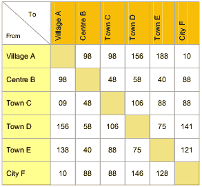
Step 1:

All travel distances between all urban centres and villages along the roads are measured.

Step 2:

The obtained travel distance can be converted into travel time by using data on speed for the various kinds of road links and transportation opportunities.

Step 3:

The distances or the time values down the columns or across the rows are summed up.

Step 4:

The urban places with the premium value supplies all others at minimized transportation costs. According to the locational values the degree of integration can be identified.

Table 1: Settlement Distance Matrix

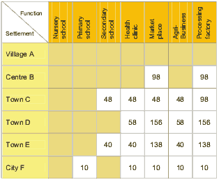
Next Opportunity Matrix

The general character of the distance matrix restricts its use and interpretation. A more detailed picture will be gained from the next opportunity matrix which combines two tools with each other; the functional matrix and the distance matrix. The rationale behind the model is the assumption that consumers minimize transportation efforts under the condition that all other factors are equal.

Step 1:

The basic idea consist in the proposal to go through the functional matrix row by row and to identify blanks or unavailable functions.

Step 2:

Then the next location to the urban place under consideration is identified within the matrix where the missing function is available.

Step 3:

The identified transportation costs are incorporated into the next opportunity matrix.

Step 4:

Going through all the functions and scanning up all the values the total interaction effort is indicated by the last column.

Table 2: Settlement Next Opportunity Matrix

The finding of the next opportunity matrix can be interpreted in
different directions:

Places with high values might be called remote areas with low access to urban facilities.
Places with low values are highly self-sufficient with locational advantages.
The overall transportation effort of one location to the facilities in other location is computed over all facilities in the following way:
Distance or time x target group x frequency x unit costs = average cost of the target group in a specific location using a specific facility in the next location.
This computation over all functions and locations provides the planners with decision criteria on the future distribution of the facilities and the allocation of investments.
The demand potential is derived from the interactions of a target group.

The results of the next opportunity matrix provides first insights into interaction patterns. The method also helps avoid complicated empirical studies. It is possible to estimate demand patterns, to distinguish between integrated and non-integrated areas to derive some ideas for the allocation of investments in connection with new infrastructure facilities.